Can you tell the nuts & berries apart in each group?
 Differentially private nuts & berries
Differential privacy, synthetic data and data anonymization have recently become very important. One big reason for this is the introduction of the GDPR policy in Europe. However, this is a complex topic. I try to give you a simple, yet hands-on introduction to how to perform data anonymization which respects the requirements differential privacy.
existing concepts
k-anonymity
K-anonymity is an established concept when reasoning about data privacy. For each group that can be identified in the data at least k non-distinguishable data points are required.
This implies that the granularity of the data needs to be reduced to fulfill the desired privacy requirements. For example, data fields such as a social security number would need to be omitted or a zip-code reduced to the first couple of digits to ensure enough data points fall within each group. I.e. when considering a data frame structured as:
zip_code, age, gender, income, level_of_education
The k-anonymization procedure whould need to ensure that at least k unique observations fall into each group to prevent the identification of any individual contained in the data.
differential privacy
Differential privacy is a much newer concept. Researchers agree that k-anonymity itself is not good enough. It turns out that prior external knowledge about that particular dataset might lead to deanonymization albeit k-anonymity. They formulate an additional requirement to the responses of a database to be statistical to prevent such issues 1. This means that the response of the database must not be exactly the same - even when executing the same query twice. To achieve this property, these methods oftentimes operate by adding random noise to the data.
❤️ combine the best of both worlds 😄
However, too much noise deteriorates the quality of the retrieved data response. An inadequate k would give either grossly coarse data or allow to deanonymize the dataset.
Instead, both methods should be combined to unite the advantages of both methods:
- tunable anonymization
- minimal noise (as needed to fulfill the privacy requirements) is added
- mathematically well-defined privacy guarantees
problem definition
Multi- or even high-dimensional data is everywhere, in particular as geospatial data is getting more and more widespread. Such kind of data is very hard to anonymize and thus finding the right methods to do so is ever more important.
For classical statistical datasets such as CRM data (=demographics) oftentimes it is deemed good enough to only anonymize the primary key (such as name, social security number) and any other PII relevant column by applying a hashing procedure where the encryption key (=salt) is deleted and coarsen the attributes to adhere to k-anonymity.
The problem with high-dimensional data is that even when rotating the salt of the PII relevant columns, secondary columns such as geolocation will still over time reveal patterns which nonetheless could make it possible to identify unique patterns and potentially de-anonymize records. This means the content must be anonymized as well to prevent such tracking over time and accidentally exposing sensitive data.
Furthermore, we need to allow for tunable anonymization guarantees to distort the data only as much as required by a specific use case to keep the quality as high as possible.
potential solutions
synthesize new data: generative adversarial networks (GANS)
A complex solution might be to synthesize fresh data. This has the advantage that even very high-dimensional data could potentially be supported. Several startups and companies offer such services nowadays. Usually, neural networks - and in particular generative adversarial networks (GANs) are applied for the data synthesis process.
However, as the size of the data which needs to be anonymized scales, graphics processing units (GPUs) need to be used - potentially in large quantity to perform the synthesis task. In a cloud-based environment, this might not be an issue as the desired hardware can be rented on an as-needed basis. However, in an on-premise data center, potentially no or only a very limited number of such special hardware might be available.
Potentially the covariance structures might be distorted. And categorical records i.e. female/male might no longer bei either or, rather 90% male and 10% female at the same time.
Lastly, one has to trust the vendor as neural networks are oftentimes considered black boxes. In this particular case, you have to trust that the learned weights of the GAN do not learn the real data by heart and therefore potentially leak sensitive information into the synthesized data.
differential privacy using approximative k-nearest neighbors
Instead, probabilistic approximative k-nearest neighbors (A-KNN) is a very simple and yet still effective method to ensure differential privacy. It is based on 100% verifiable mathematical formulas, which easily allow to argue for correctnes of anonymization procedure and you do not have to trust that the black box GAN simply just works ™. By combining the aforementiond concepts of k-anonymity with differential privacy we can combine the best of both worlds 23. Only a minimal required noise needs to be added whilst still keeping the data anonymized. Firstly, the k nearest neighbors are retrieved. Then, the maximal distance to the point furtherst away is considered to parametrise the process which adds only the requried amount of Gaussian noise to the data.
Furthermore, as the k in KNN is tunable the desired level of anonymization can be calibrated easily. Therefore the data is only minimally distorted whilst still strictly mathematically guaranteeing the desired level of privacy.
example
In the following section, I will outline an example of how to perform the A-KNN computation and evaluate the quality degradation of the anonymized data.
For a key, one geospatial point needs to be anonymized. As latitude and longitude are present a two dimensional KNN index needs to be created.
tuning parameters
For the sake of this example, we will assume an initial k-anonymity of 5. Therefore, 5 keys have the identical geospatial point and searching for a specific key based on this point results in a probability for a true match of 20%.
When statistically verifying this assumption we need to sample a large number of runs and we need to ensure that up to or even better less than this probability of a real match (the original point is detected).
Due to the nature of the Gaussian, the real point may be far more shifted outside the boundary defined by k.
The two important tuning parameters are:
- k to determine the knn.
- sigma: the standard deviation of the gaussian noise (estimated according to the particular k-nearest neighbors)
reproducibility
To make the example easily reproducible a conda environment is created.
Create a file named environment.yml with the following contents:
name: aknn
channels:
  - conda-forge
  - defaults
dependencies:
  - jupyterlab
  - pandas
  - scipy
  - numpy
  - seaborn
  - python >= 3.8
Then, apply it by executing:
conda env create -f environment.yml
the code
We begin by importing the required python libraries.
%pylab inline

import pandas as pd
import numpy as np
from scipy.spatial import cKDTree
import seaborn as sns; sns.set()
Then create some dummy data:
rng = np.random.RandomState(0)

n_points = 20
d_dimensions = 2

X = rng.random_sample((n_points, d_dimensions))

df = pd.DataFrame(X).reset_index(drop=False)
df.columns = ['id_str', 'lat1', 'long1']
df.id_str = df.id_str.astype(object)
df.head()
| id_str | lat1 | long1 | |
|---|---|---|---|
| 0 | 0 | 0.548814 | 0.715189 |
| 1 | 1 | 0.602763 | 0.544883 |
| 2 | 2 | 0.423655 | 0.645894 |
| 3 | 3 | 0.437587 | 0.891773 |
| 4 | 4 | 0.963663 | 0.383442 |
As a next step, we must create a multidimensional index to efficiently query for the k-nearest neighbors.
For this, a cKDTree from the awesome scipy library is used.
k_neighbours = 10

def construct_tree(df, features, leaf_size=4):
    return cKDTree(df[features], leafsize=leaf_size)


def get_neighbors_and_ARGMAX_distance(tree, X_query, k_neighbours, workers=-1):
    dist,ind = tree.query(X_query, k=k_neighbours +1,workers=workers)
    return dist[:, -1]


def get_neighbors_and_ARGMAX_distance_debug(tree, X_query, k_neighbours, workers=-1):
    k_neighbours = k_neighbours + 1
    dist,ind = tree.query(X_query, k=k_neighbours,workers=workers)
    X_query_no_self = np.delete(X_query[ind], 0, 1)
    dist_no_self = np.delete(dist, 0, 1)
    argmax_distance = dist[:, -1]
    return X_query_no_self, dist_no_self, argmax_distance


tree = construct_tree(df,['lat1', 'long1'])
X_query, distance_matrix_neighbors, argmax_distance = get_neighbors_and_ARGMAX_distance_debug(tree, X, k_neighbours, workers=-1)

df['complex_type'] = list(X_query)
df['dist_same_order'] = list(distance_matrix_neighbors)

# as it is sorted - the last element === ARGMAX
df['max_distance'] = distance_matrix_neighbors[:, -1]
display(df.head(n=3))
For debugging purposes, we store all the suggested k neighbors, their distances and the maximum distance.
| id_str | lat1 | long1 | complex_type | dist_same_order | max_distance | |
|---|---|---|---|---|---|---|
| 0 | 0 | 0.548814 | 0.715189 | [[0.46147936225293185, 0.7805291762864555], [0.6120957227224214, 0.6169339968747569], [0.4236547993389047, 0.6458941130666561], [0.45615033221654855, 0.5684339488686485], [0.6027633760716439, 0.5448831829968969], [0.4375872112626925, 0.8917730007820798], [0.5680445610939323, 0.925596638292661], [0.7781567509498505, 0.8700121482468192], [0.26455561210462697, 0.7742336894342167], [0.521848321750... | [0.10907127514430776, 0.1168706843085668, 0.14306129268590195, 0.17356156244458887, 0.1786470956951876, 0.20869371845180915, 0.21128429576441266, 0.2767099903186786, 0.2903253022891915, 0.3017347428745624] | 0.301735 |
| 1 | 1 | 0.602763 | 0.544883 | [[0.6120957227224214, 0.6169339968747569], [0.45615033221654855, 0.5684339488686485], [0.5218483217500717, 0.4146619399905236], [0.5488135039273248, 0.7151893663724195], [0.7917250380826646, 0.5288949197529045], [0.4236547993389047, 0.6458941130666561], [0.46147936225293185, 0.7805291762864555], [0.9437480785146242, 0.6818202991034834], [0.7781567509498505, 0.8700121482468192], [0.568044561093... | [0.07265268387659406, 0.14849250217301266, 0.15331281142157657, 0.1786470956951876, 0.18963684840116496, 0.20562852490057235, 0.2747548119945285, 0.36745386250210593, 0.369420735741312, 0.3822932528265394] | 0.382293 |
| 2 | 2 | 0.423655 | 0.645894 | [[0.45615033221654855, 0.5684339488686485], [0.46147936225293185, 0.7805291762864555], [0.5488135039273248, 0.7151893663724195], [0.6120957227224214, 0.6169339968747569], [0.26455561210462697, 0.7742336894342167], [0.6027633760716439, 0.5448831829968969], [0.4375872112626925, 0.8917730007820798], [0.5218483217500717, 0.4146619399905236], [0.11827442586893322, 0.6399210213275238], [0.5680445610... | [0.08400021841986086, 0.1398474090136695, 0.14306129268590195, 0.19065327150479405, 0.2044103672537493, 0.20562852490057235, 0.24627330250392146, 0.251217606287901, 0.3054387832702051, 0.3147727845883083] | 0.314773 |
Now following a worst-case assumption we use the largest distance (max_distance) as the standard deviation when parametrizing the Gaussian.
np.random.seed(1)
columns_to_be_sampled = ['lat1', 'long1']
synth_string = 'sythesized'

df = df.drop(['complex_type', 'dist_same_order'], axis = 1)

def sample_gauss(mean, sigma):
    return np.random.normal(mean, sigma)


def sample_multiple(df, columns_to_be_sampled, sigma):
    for col_sample in  columns_to_be_sampled:
        df[f'{col_sample}_{synth_string}'] = sample_gauss(df[col_sample], df[sigma])
    return df

df = sample_multiple(df, columns_to_be_sampled, 'max_distance')
df.columns = sorted(df.columns)
df.head()
| id_str | lat1 | lat1_sythesized | max_distance | long1 | long1_sythesized | |
|---|---|---|---|---|---|---|
| 0 | 0 | 0.548814 | 0.715189 | 0.301735 | 1.038935 | 0.383094 |
| 1 | 1 | 0.602763 | 0.544883 | 0.382293 | 0.368893 | 0.982503 |
| 2 | 2 | 0.423655 | 0.645894 | 0.314773 | 0.257401 | 0.929690 |
| 3 | 3 | 0.437587 | 0.891773 | 0.384208 | 0.025344 | 1.084835 |
| 4 | 4 | 0.963663 | 0.383442 | 0.600408 | 1.483261 | 0.924323 |
validation
When evaluating we must ensure that a single run of the anonymization process outputs strictly anonymized data. On the other hand, we further must check that many subsequent runs of the anonymization procedure result in unique datasets that would not be traceable to a single identity.
We use the root mean square error (RMSE) to evaluate the difference in quality by calculating the distance metric and evaluating total shift distance in the euclidean space, which in the case of this example has two dimensions named: lat1, long1 referring to a (y,x) coordinate tuple of latitude and longitude.
In a real-world scenario, you will have to deal with coordinate systems. Usually, this means using a Haversine distance on coordinates in
epsg:4326WGS-84 projection or simply reprojecting to a (locally) euclidean coordinate system.
The overall distance in all two dimensions:
$$distance_{combined} = \sqrt{ (lat_1 - lat_{1new})^2 + (long_1 - long_{1new})^2}$$single-run anonymization
When evaluating the closest match according to the distance metric and comparing it with the original point we will evaluate if reverse engineering was possible or not in a binary way, i.e. whether a best match will resolve to the same original data point.
Even in cases where this is happening, it is not a problem at all as this case would not be clear to anyone trying to de-anonymize the data set. In fact we do expect some true matches with up to the the rate of $\frac{1}{k}$.
def comparison_function_sample(r):
    if r.lat1 == r.closest_match[0]:
        if r.long1 == r.closest_match[1]:
            return 1
        else:
            return 0
    else:
        return 0


def simulate_single_iteration(sim_data, X_sim, i):
    tree = construct_tree(sim_data,columns_to_be_sampled)
    sim_data['max_distance'] = get_neighbors_and_ARGMAX_distance(tree, X, k_neighbours, workers=-1)
    sim_data = sample_multiple(sim_data, columns_to_be_sampled, 'max_distance')
    sim_data['iteration'] = i

    # validate quality by searching for the closest match for the randomly sampled (synthesized point)
    # by looking at the next/closest raw/original point. Assume that one is a match (i.e. the exact orignal)
    # iff (if and only if) all dimensions exactly match up
    synthesized_columns = sim_data.columns[sim_data.columns.str.contains(synth_string)]
    X_sim = sim_data[synthesized_columns].values
    _, ind=tree.query(X_sim, k=1,workers=-1)
    sim_data['closest_match'] = list(X[ind])

    # compare original with sampled, where closest_match contains the sample
    sim_data['bad_true_match'] = sim_data.apply(comparison_function_sample, axis=1)
    return sim_data
multi-run anonymization
Here, it is required to show that repeated execution of the anonymization procedure generates fresh data points each time and thus successfully prevents tracking of a user over time.
As we want to be able to analyze the data over multiple runs we must re-create the initial dataset and ensure we store the number of the run additionally when executing the simulation multiple times.
def simulate_iteration(iterations, sim_data, X_sim):
    iteration_results = []

    for i in range(1, iterations +1):
        i_result = simulate_single_iteration(sim_data.copy(), X_sim, i)
        iteration_results.append(i_result)
    return pd.concat(iteration_results)

result = simulate_iteration(3, df, X)
results
As described before we calculate the RMSE of the multi-dimensional distance.
Potentially, a Mahalanobis distance could be used to compute robust multivariate distances. However, this might add considerable compute time to the calculation.
result['d_combined'] =  np.sqrt(np.sum(np.array([(result.long1 - result.long1_sythesized) **2,
                         (result.lat1 - result.lat1_sythesized) **2]), axis=0))
result.d_combined.plot.hist()
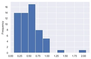
We can observe that for a large part of the data the shift is small.
Within a single day the number of potential re-identifications is alredy very low:
for i in result['iteration'].unique():
    print(i)
    print(result[result['iteration'] == i].bad_true_match.value_counts(normalize=True))
1
0    0.95
1    0.05
Name: bad_true_match, dtype: float64
2
0    0.85
1    0.15
Name: bad_true_match, dtype: float64
3
0    0.8
1    0.2
Name: bad_true_match, dtype: float64
And we observe that it is consistently low and maximally up to the aforemationed ratio of: $\frac{1}{k}$. The reader has to keep in mind that this means identification by random chance. Even if the identification might be possible sometimes - in a real-world scenario where the true labels will not be present in the data, even identifying a random match will be much harder.
This number is further reduced when trying to identify a user over time.
To better understand the effect, let`s visualize the outcome.
r = result[['id_str', 'lat1', 'long1', 'lat1_sythesized','long1_sythesized','iteration']]
display(r.head(n=2))

rx = r[['id_str', 'lat1', 'long1', 'iteration']].copy()
rx['kind'] = 'regular'

rx = pd.concat([rx, r[['id_str', 'lat1_sythesized', 'long2_sythesized', 'iteration']]], axis=0)


rx['kind'] = rx['kind'].fillna('sythesized')
rx.location1 = rx.lat1.fillna(rx.lat1_sythesized)
rx.location2 = rx.long1.fillna(rx.long1_sythesized)
rx = rx.drop(['lat1_sythesized', 'long1_sythesized'], axis= 1)

rx = rx[(rx.kind=='regular') & (rx.iteration == 1) | (rx.kind == 'sythesized')]
plt.figure(figsize=(16, 9))
sns.set_style("ticks")
sns.scatterplot(x="location1", y="location2", data=rx[rx.kind =='regular'], hue='kind', s=80)
sns.despine()
We visualize the result by simply plotting the original points. Next to the original points, the synthesized observations are plotted for a single iteration.
plt.figure(figsize=(16, 9))
sns.set_style("ticks")
sns.scatterplot(x="lat1", y="long1", data=rx[(rx.iteration == 1)], hue='kind', s=80)
sns.despine()
The freshly randomly generated observations are marked in orange, the original data in blue.
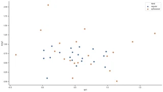
One might assume that synthesized data is the closest true match to the next blue original point. But this indeed is false due to the Gaussian noise applied to the data.
plt.figure(figsize=(16, 9))
sns.set_style("ticks")
sns.scatterplot(x="location1", y="long1", data=rx, hue='kind', style='iteration', s=80)
sns.despine()
Furthermore, we must show that the generated data is differentially private i.e. stochastic and not returning equal values.
plt.figure(figsize=(16, 9))
sns.set_style("ticks")
sns.scatterplot(x="location1", y="long1", data=rx[rx.kind == 'sythesized'], hue='id_str', style='iteration', s=80)
sns.despine()
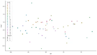
As a result profiling a user over multiple runs of the anonymization procedure becomes very unlikely. In fact, it turns out that with the aforementioned parameters the probability is 4% to track a user from one run to the next one. To track a user over multiple runs the probabilities need to be multiplied - and very quickly become very small, in fact close to 0.
Furthermore, the described procedure is optimal, in the sense that only minimal noise is added to achieve the desired level of privacy.
q = result.d_combined.quantile([.1, .2, .3, .4, .5, .6, .7, .8, .9, .99])
q.plot()
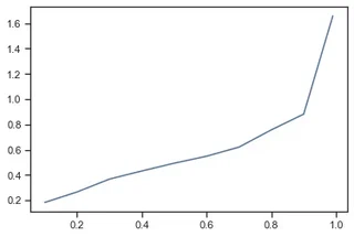
when analyzing the shift of the data using percentiles it turns out that for more than 80% the shift is rather minimal!
summary

Can you tell the differentially anonymized berries apart?
Similarly to the nuts and berries in the picture, the generated anonymized data is ensuring the privacy of the individual item. It is impossible to tell individual identities appart.
We have shown how to easily create truly & also 100% mathematically provable anonymized data for complex high-dimensional real-world data sets such as geospatial data.
For simplicity, only 2D anonymization has been shown here. Certainly, even much higher dimensional data can be anonymized efficiently in the same way. However, there is a limit to the efficiency of the multidimensional index due to the curse of dimensionality 4.
In order to improve the scalability of this approach, approximate indices such as https://github.com/spotify/annoy or https://github.com/facebookresearch/faiss might come handy. Alternatively, accelerator chips such as GPUs could be used to improve the KNN matching. Nvidia claims that by using RAPIDS cuml they could achieve a speed-up of 600x
disclaimer
Privacy is like IT security - given an adversary with enough interest in pawning you and enough resources it will always work to find a security hole.
The quality of the anonymization approch clearly depends on the selected parameters (k, sigma).
The source of the nuts & berry image is based on the automated AI-based design suggestions of Microsoft Powerpoint.
Smith, 2012: Pinning down privacy in statistical databases ↩︎
Domingo-Ferrer, 2006: Microaggregation for Database and Location Privacy ↩︎
Soria-Comas, 2014: Enhancing Data Utility in Differential Privacy via Microaggregation-based k-Anonymity ↩︎
Aggrawarl, 2005: On k-Anonymity and the Curse of Dimensionality ↩︎
